What can you do with time-series data?
What time-series data is, where it comes from, how machine learning puts it to work, and what return to expect from it.
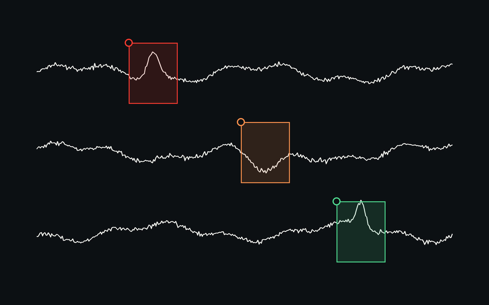
A time series is a sequence of measurements ordered in time: the vibration of a bearing sampled a thousand times a second, the temperature of a satellite every ten seconds, the pressure in a pipe every minute. What can be done with one depends less on the algorithm than on the labels: with events named and marked by people who know the machine, a series can be searched, classified, monitored and forecast. Without them, it can only be described.
What a time series is
Each row is an instant and one or more values. The sampling is regular when the instants are equally spaced, irregular otherwise; the series is multivariate when several sensors are read at each instant. Four rows of a two-sensor series:
| Time | Current (A) | Vibration (g) |
|---|---|---|
| 2026-09-22T08:00:01Z | 12 | 0.2 |
| 2026-09-22T08:00:02Z | 13 | 0.1 |
| 2026-09-22T08:00:03Z | 16 | 0.3 |
| 2026-09-22T08:00:04Z | 14 | 0.4 |
The sampling rate decides what can be seen. A signal sampled fs times a second shows nothing above fs/2 (Shannon, 1949): a temperature read every minute cannot show a vibration at 50 Hz, and an audio recording at 200 kHz is a time series like any other, only much faster. Acoustic recordings, radio recordings and distributed acoustic sensing are all time series at high rate, and the same questions apply to them.
Where it comes from
Almost every machine that runs produces one: the sensors of an engine on a test bench, the telemetry of a satellite, the current and vibration of a pump, the hydrophones of a mooring, the strain along an optical fibre. The volumes are large and the interesting parts are rare: on a test bench, a few abnormal observations in hours of high-frequency signal; on a radio site, one fault among thousands of normal measurements.
Five things you can do with it
| Task | The question | What it needs |
|---|---|---|
| Labeling | Where are the events, and what are they? | A taxonomy, specialists, a reviewed dataset |
| Anomaly detection | Where does the series stop behaving as it should? | Examples of the normal, and of the anomalies when they are known |
| Classification | Which kind of event is this? | Labeled events of each kind |
| Similarity search | Where else does this pattern appear? | One labeled example and a distance: dynamic time warping (Sakoe and Chiba, 1978) or the matrix profile (Yeh et al., 2016) |
| Forecasting, remaining useful life | What comes next, and how long before the failure? | Series recorded up to the failure, such as NASA's C-MAPSS engines (Saxena et al., 2008) |
The first task feeds the four others. Similarity search is the shortcut: from a single event an analyst has marked, the ranges that resemble it are found across the other series and reviewed one by one, which is how a dataset of rare events grows from one example to hundreds.
What it takes to start
- Data in a readable form. CSV with an ISO 8601 timestamp column and one column per sensor is enough. Units and sampling rates are written down; a series split across files by machine or by day is joined by an identifier.
- The events, named. A short taxonomy of what matters: the fault, the transient, the drift, the artefact of the bench. It is written with the people who run the machine.
- A first labeled sample. A few recordings labeled and reviewed, enough to search the rest by similarity and to judge a first detector.
- Computed columns. A derivative, a low-pass filter, a normalisation, or the time left before the next labeled event, which is the target of a remaining-useful-life model.
- Partitions and versions. Training, validation and test sets fixed once, and the dataset frozen in a version a model can be traced to.
Where Ezako applies it
Ezako has worked on the high-frequency sensor series of engine development tests with Safran Aircraft Engines (2021), on satellite telemetry for CNES (2020), on the ranking of more than 76,000 radio sites for inspection with ANFR (2020), and on fault detection on a microcontroller within the DeepGreen project led by CEA (2023). Upalgo Labeling Timeseries is the desktop application built for this work: CSV files of up to 1,000 series each, events as ranges or points, similarity search across series, label candidates proposed from rare patterns, and computed columns, all on the workstation. The software and the application page give the details.
Sources
- C. E. Shannon, Communication in the Presence of Noise, Proceedings of the IRE 37(1), 1949.
- H. Sakoe, S. Chiba, Dynamic Programming Algorithm Optimization for Spoken Word Recognition, IEEE Transactions on Acoustics, Speech, and Signal Processing 26(1), 1978.
- C.-C. M. Yeh et al., Matrix Profile I: All Pairs Similarity Joins for Time Series, IEEE ICDM, 2016.
- A. Saxena, K. Goebel, D. Simon, N. Eklund, Damage Propagation Modeling for Aircraft Engine Run-to-Failure Simulation, IEEE PHM, 2008.
- Ezako, projects.
First published in June 2022; rewritten in September 2026 around the labels, the five tasks, what a project starts with and the projects carried out. The unsourced count of sensors in the world was removed.