What is MTBF, and why does it matter?
The mean time between failures says how reliable a machine is: what it is, why it matters, how to calculate it and how to improve it.
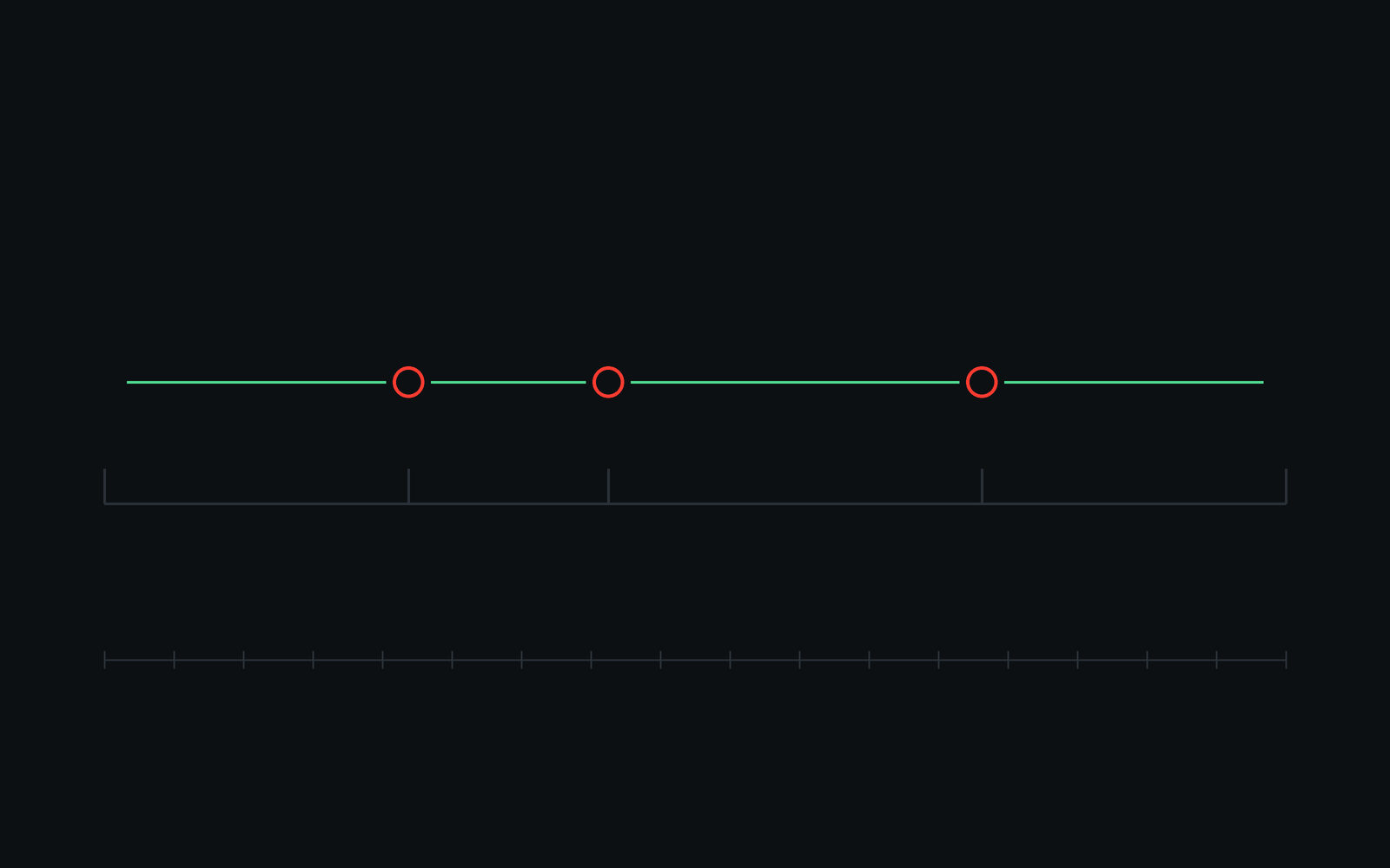
The mean time between failures, MTBF, is the total operating time of a repairable item divided by the number of failures it had over that time. It says how often a machine fails, on average, over a period; it does not say how long a given machine will run before its next failure, and it is only as good as the count of failures behind it.
What it is, and what its neighbours are
The dependability vocabulary of the IEC (IEC 60050-192) defines the family of indicators together, and the distinctions matter.
| Indicator | Applies to | Definition |
|---|---|---|
| MTBF | A repairable item | Mean operating time between failures |
| MTTF | A non-repairable item | Mean operating time to failure, its life |
| MTTR | A repairable item | Mean time to restoration, from failure to return to service |
| Availability | A repairable item | MTBF divided by the sum of MTBF and MTTR: the share of the time the item can do its job |
Operating time is the time the item runs, not calendar time: a pump idle for a weekend gains no operating hours. A failure is an event defined in advance, the end of the item's ability to perform its function; a maintenance stop is not one.
How to calculate it
MTBF = operating hours in the period / number of failures in the period.
A pump is scheduled for a 12-hour shift. It runs 10 hours, fails 4 times, and the 4 repairs take 2 hours in all.
- MTBF = 10 / 4 = 2.5 hours.
- MTTR = 2 / 4 = 0.5 hour.
- Availability = 2.5 / (2.5 + 0.5) = 83.3 %.
The same arithmetic over a fleet gives a fleet MTBF: 40 pumps with 20,000 operating hours and 16 failures give 1,250 hours between failures, for the fleet. No single pump is promised 1,250 hours.
What it does not say
- It is not a lifetime. When failures arrive at a constant rate, the probability that an item runs its whole MTBF without failing is e-1, 36.8 %. Two items out of three fail before the MTBF; the average is pulled up by the ones that run long.
- It assumes a constant rate. The failure rate of most equipment is not constant: higher at the start, when defects of manufacture show, and at the end, when parts wear out. A single MTBF over the life of an item hides both.
- A predicted MTBF is not a measured one. Handbook methods such as MIL-HDBK-217F (1991, notice 2 of 1995) sum the predicted failure rates of components; they are a design tool, and field data regularly diverge from them by a large factor. A figure on a datasheet says which method produced it, or it says little.
- It depends on the count. Two sites that count failures differently produce MTBFs that cannot be compared. ISO 14224, on the collection and exchange of reliability and maintenance data, exists for that reason: a taxonomy of equipment, of failure modes and of what counts as a failure.
How to improve it
- Count the same way everywhere. Write down what a failure is for each class of equipment, and record every one with its date, its mode and its repair time. The MTBF becomes comparable between sites and between years.
- Look at the series before the failure. Most failures are preceded by a change in the sensors of the machine: vibration, temperature, current, pressure. Marking each failure on the recorded series, and the hours before it, turns a count into a labeled dataset.
- Move from intervals to remaining useful life. With enough labeled failures, a model estimates for each machine the time left before the next one, instead of a fleet average. The reference dataset for this problem is NASA's C-MAPSS (Saxena et al., 2008): turbofan engines simulated to failure, 21 sensors each, in four fleets.
- Validate at an operating point. An estimate that is wrong often costs unnecessary stops; one that is late costs failures. The model is judged on held-out machines, at the precision and the lead time the maintenance plan needs, before it changes anything in the plan.
In Upalgo Labeling Timeseries, an engineer marks the failures on the series of a fleet, and a computed column gives, at each point, the remaining time before the next labeled event: the target a remaining-useful-life model is trained on. The software and the sensor data analysis page describe the workflow.
Sources
- IEC, IEC 60050-192, International Electrotechnical Vocabulary, part 192: dependability, 2015.
- US Department of Defense, MIL-HDBK-217F, Reliability Prediction of Electronic Equipment, 1991, notice 2, 1995.
- ISO, ISO 14224:2016, Petroleum, petrochemical and natural gas industries: collection and exchange of reliability and maintenance data for equipment, 2016.
- A. Saxena, K. Goebel, D. Simon, N. Eklund, Damage Propagation Modeling for Aircraft Engine Run-to-Failure Simulation, IEEE PHM, 2008.
First published in May 2022; rewritten in September 2026 with the IEC definitions, a corrected example, what the indicator does not say, and the way from a count of failures to a remaining-useful-life model.