What is supervised anomaly detection?

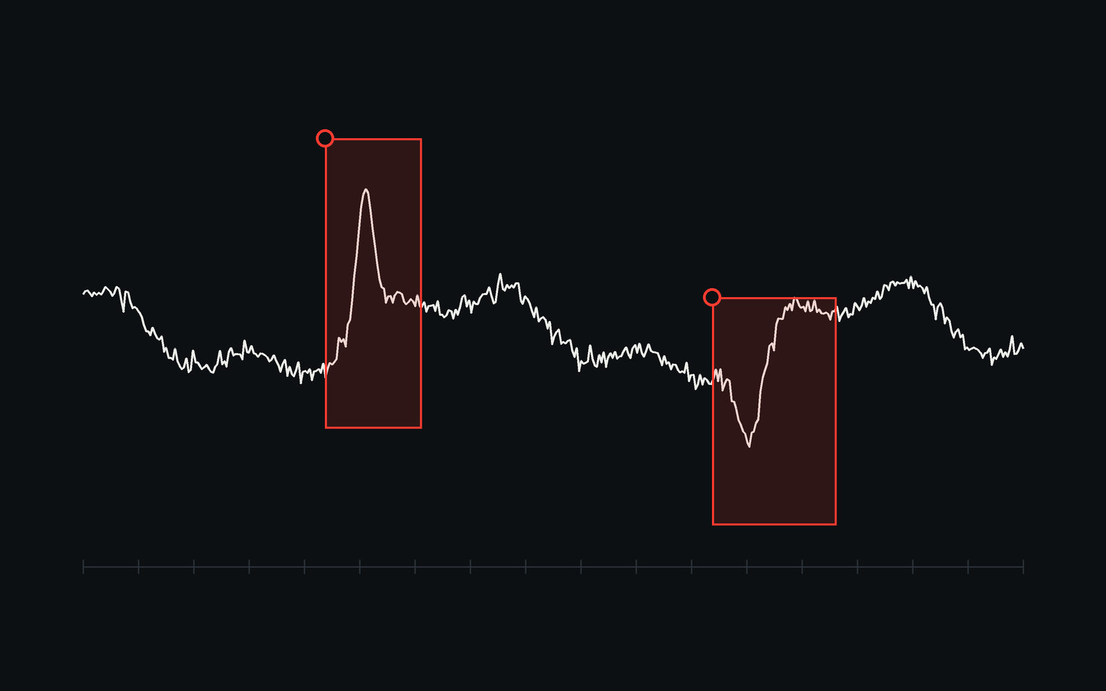
Supervised anomaly detection trains a model on recordings where specialists have already marked which events are normal and which are not, then lets the model find the same kinds of events in new data. It is the most precise of the three settings of anomaly detection, and the most demanding: it needs a labeled dataset, built and reviewed before any model is trained.

Three settings, one question

The reference survey of the field (Chandola, Banerjee and Kumar, 2009) distinguishes anomaly detection by what the training data says about each observation.

Setting	What the labels say	What the model finds	Typical methods
Supervised	Normal and anomalous, on every training example	The kinds of anomalies it was shown	Classifiers: gradient-boosted trees, convolutional networks on spectrograms, recurrent networks on series
Semi-supervised	Normal only	Anything that departs from the normal it learned	One-class SVM (Schölkopf et al., 2001), autoencoders
Unsupervised	Nothing	What is rare or isolated in the data	Isolation Forest (Liu, Ting and Zhou, 2008), clustering, distance to neighbours

The three are not competitors. An unsupervised method is how a team screens an archive it knows nothing about; a semi-supervised one is how it monitors a machine whose faults have not happened yet; a supervised one is what it builds once analysts have named the events that matter and marked enough of them.

What it takes

A supervised detector is only as good as its labels. Four things decide the result before any training run.

• A taxonomy. The events are named before they are marked: a vessel passage, a whistle, a sensor drift, a test-bench artefact. Two analysts who label the same recording must produce the same labels; the review between them is part of the dataset.
• Rare positives. Anomalies are rare by definition, so the training set is imbalanced. The remedies are known: rebalancing the classes, weighting the loss, and above all judging the model on precision and recall rather than on accuracy. On a set where 1 event in 1,000 is anomalous, a model that flags nothing is 99.9 % accurate and useless.
• The right curve. When positives are rare, the precision-recall curve says more than the ROC curve, which stays flattering as the negatives pile up (Saito and Rehmsmeier, 2015). On a continuous stream, the operating point is read as false alarms per hour at a given recall.
• A frozen dataset. Training, validation and test partitions are fixed once, stratified by class or split by blocks of time so that a model is never tested on the neighbours of what it learned. Each version is immutable: a model is traceable to the exact data it saw.

How it runs, step by step

1. Specialists label a first sample of recordings against the taxonomy, with a reviewer checking each file.
2. The labels are partitioned into training, validation and test sets, and a hold-out set is kept aside.
3. A model is trained on the training set and its operating point is chosen on the validation set: the threshold that gives the precision the operation requires.
4. The test set gives the figures that will be quoted: precision, recall and false alarms per hour at that threshold.
5. In service, the model proposes and an analyst decides. Every detection is validated or rejected, and each decision becomes a new label.
6. The dataset is versioned again with the new labels, and the model retrained: the loop is what makes the detector improve on the customer's own data.

Where Ezako applies it

Ezako has worked in this setting on several kinds of signals. In 2020, CNES entrusted it with the detection of anomalies in satellite telemetry, alongside the conventional surveillance methods. The same year, for ANFR, it predicted which radio sites were most likely to reveal an anomaly, to order the inspections of a national park of more than 76,000 sites. In 2021, with Safran Aircraft Engines, it published a deep learning approach to abnormal observations in the high-frequency sensor series of engine development tests. In 2023, within the DeepGreen project led by CEA, it worked on fault detection by machine learning on a microcontroller.

The tooling follows the method. In Upalgo Labeling Timeseries, an analyst marks an event on a series, searches the other series for the ranges that resemble it, and reviews each candidate before it receives a label; rare patterns of a column are proposed as label candidates. UpalgoDB keeps the labels, builds the partitioned datasets in immutable versions, and runs the detectors on the customer's infrastructure, offline. The algorithms, the datasets and the labeling service describe what is available.

Sources

• V. Chandola, A. Banerjee, V. Kumar, Anomaly Detection: A Survey, ACM Computing Surveys 41(3), 2009.
• T. Saito, M. Rehmsmeier, The Precision-Recall Plot Is More Informative than the ROC Plot When Evaluating Binary Classifiers on Imbalanced Datasets, PLOS ONE 10(3), 2015.
• F. T. Liu, K. M. Ting, Z.-H. Zhou, Isolation Forest, IEEE ICDM, 2008.
• B. Schölkopf et al., Estimating the Support of a High-Dimensional Distribution, Neural Computation 13(7), 2001.
• Ezako, A deep learning approach to signal anomaly detection, with Safran Aircraft Engines, 2021; projects.

First published in December 2020; rewritten in September 2026 with the three settings, the metrics for rare events, the steps of a supervised project and the projects carried out since.